AMA1007 : Calculus and Linear Algebra
2022-2023
Second Semester.
Please
refer to Blackboard and look under “Content” for listing of zoom recordings of
lectures (zoom recordings of lectures will be uploaded to Panopto within one or
two days right after each lecture).
Students
could also find ALL the pre-recorded lecture videos in Panopto useful to view
at any time (videos can only be viewed via Panopto for officially registered
AMA1007 students).
The pace
for lectures usually is about 40 to 50 pages of lecture notes per a 2-hour
session. It is recommended for students to read the relevant lecture materials
as well as to watch the pre-recorded video clips beforehand prior to joining the lectures.
All students should watch all the four demo
videos on CoCalc.
- Course
Outline (a pdf file).
- The prerequisite for this subject is HKDSE
M1/M2, or AMA1100. The prerequisite requirement is strictly enforced. Students
not having the prerequisite requirement are not allowed to take the
subject.
- Under
the current pandemic situation, students MUST wear proper face mask (and
wear it PROPERLY) at all times in class.
- Under
the current pandemic situation, students MUST keep the official
recommended social distance with each other (at least 1 meter).
- Under
the current pandemic situation, students MUST NOT get near to any teaching
team members less than the official recommended social distance (at least
1 meter) (for example, do not approach Subject Lecturer immediately after
lecture, but reach Subject Lecturer via Zoom Chat instead).
·
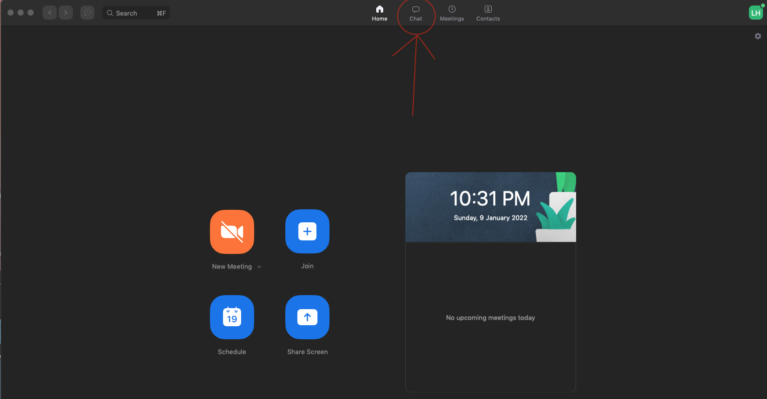
Students
should be using the official PolyU student zoom account to communicate via Zoom
Chat (image) with the
subject lecturer. Zoom Chat is a built-in instant messaging function in zoom. For
the first time, student should state clearly the name of the subject, the
student name, as well as the student id, and student cannot change their zoom
account name originally set by PolyU/ITS for all AMA1007 matters. Note that, pure plain keyboard
texting is not an effective way to communicate maths questions, as students
cannot formulate the questions properly to ask teaching team members without
maths symbols, and teaching team members cannot answer effectively without a
whiteboard (when most students do not know latex). Thus, Zoom
video sessions with the use of zoom whiteboard functions would be preferred.
Extra zoom sessions
priority will only be given to students who have watched all the four CoCalc
demo videos completely, and watched the relevant pre-recorded lecture videos,
according to the Panopto viewing record. Throughout the semester, Subject
Lecturer may contact students individually using the Zoom Chat functions only. Students should set up their
Zoom account properly and accept the Zoom Contact Invitation by the Subject
Lecturer whenever they receive one.
· To
establish Zoom Chat with the Subject Lecturer, see Blackboard and go to the
sign-up sheet under “Groups” to indicate you would like to receive a Zoom
Contact invitation from the Subject Lecturer.
- The delivery mode of the subject is 1
two-hours lecture and 1 one-hour tutorial per teaching week (students can
only join their own tutorial group).
o
Pre-recorded
lecture video: page
009-014
o
Pre-recorded
lecture video: page
015-025
o
Pre-recorded
lecture video: page
026-039
o
Pre-recorded
lecture video: page
040-062
§ and checking the example on page
42 with CoCalc Jupyter (polynomial long division, partial fraction, 2D-plot)
o
Pre-recorded
lecture video: page
063-082
§ and checking the example on page
70 with CoCalc Jupyter (piecewise define function, taking limits from
positive or negative sides, 2D-plot)
§ and checking the example on page
76 with CoCalc Jupyter (taking limits, 2D-plot)
o
Pre-recorded
lecture video: page
083-126
§ and checking the example on page
109 with CoCalc Jupyter (taking limit to singularity point from positive or
negative sides)
§ and checking the example on page
121 with CoCalc Jupyter (taking limit to positive infinity or to negative
infinity)
§ and checking the example on page
126 with CoCalc Jupyter (taking limit to positive infinity)
o
Pre-recorded
lecture video: page
127-128
o
Pre-recorded
lecture video: page
129-156
§ and checking the example on page
132 with CoCalc Jupyter (plot of Unit-Step Function (Heaviside Function)
and taking limit)
o
Pre-recorded
lecture video: page
157
o
Pre-recorded
lecture video: page
158-196
§ and checking the example on page
173 with CoCalc Jupyter (differentiate symbolically)
§ and checking the example on page
184 with CoCalc Jupyter (differentiate symbolically)
§ and checking the plot of example on page
191 with CoCalc Jupyter (implicit plot and implicit differentiation)
§ and checking the example on page
196 with CoCalc Jupyter (differentiate n times)
o
Pre-recorded
lecture video: page
197-228
o
Pre-recorded
lecture video: page
229-257
§ another example
with CoCalc Jupyter to find inflection points of a rational function
o
Pre-recorded
lecture video: page
258-279
§ and checking the example on page
266 with CoCalc Jupyter (integrate symbolically)
o
Pre-recorded
lecture video: page
280-302
§ and checking the example on page
290 with CoCalc Jupyter (integrate symbolically)
§ and checking the example on page
294 with CoCalc Jupyter (integrate symbolically, with a, b)
§ and checking the example on page
302 with CoCalc Jupyter (integrate symbolically, with n)
o
Pre-recorded
lecture video: page
303-324
§ and checking the example on page
308 with CoCalc Jupyter (integrate rational function)
§ and checking the example on page
323 with CoCalc Jupyter (definite integral)
§ Two
more examples on integration.
o
Pre-recorded
lecture video: page
325-365
o
Pre-recorded
lecture video: page
329a
§ and checking the example on page
361 with CoCalc Jupyter (Volume of rotation)
§ and checking the example on page
365 with CoCalc Jupyter (Arc-Length)
o
Pre-recorded
lecture video: page
366-372
§ and checking the example on page
368 with CoCalc Jupyter (Improper Integral Type 1, taking limit to
infinity)
§ and checking the example on page
371 with CoCalc Jupyter (Improper Integral Type 2, taking limit to
singularity)
o
Pre-recorded
lecture video: page
373-384
§ and checking the example on page
374 with CoCalc Jupyter (Infinite Series, infinite sum of numbers)
§ and checking the example on page
379 with CoCalc Jupyter (Infinite Series, using Sage Symbolic sum)
o
Pre-recorded
lecture video: page
385-393
§ and checking the example on page
388 with CoCalc Jupyter (Infinite sum, and differentiate term-by-term to
form another series, and check)
§ and checking the examples on page
391 with CoCalc Jupyter (Maclaurin expansions, and check)
§ Supplementary
Notes on finding the Power Series expression of a Rational Function without
using the Taylor/Maclaurin technique and check
with CoCalc.
o
Pre-recorded
lecture video: page
393-399
o
Pre-recorded
lecture video: page
400-415
§ and checking the example on page
407 with CoCalc Jupyter (determinant)
§ and checking the example on page
415 with CoCalc Jupyter (determinant)
o
Pre-recorded
lecture video: page
415a
o
Pre-recorded
lecture video: page
415b
o
Pre-recorded
lecture video: page
416-425
§ and checking the example on page
418 with CoCalc Jupyter (solving linear system)
§ and checking the example on page
422 with CoCalc Jupyter (finding values of k that make determinant = 0)
o
Pre-recorded
lecture video: page
425a-425b
§ and checking the example on page
425b with CoCalc Jupyter (box product (volume of
parallellepiped) and 3D plot)
§ Supplementary
notes on using Determinant to check if 3 points in 2D are collinear (contained
in one straight line) and
check
with CoCalc.
o
Pre-recorded
lecture video: page
426-434
o
Pre-recorded
lecture video: page
435-445
§ and checking the example on page
437 with CoCalc Jupyter (matrix multiplication)
o
Pre-recorded
lecture video: page
445a
o
Pre-recorded
lecture video: page
446-452
§ and checking the example on page
448 with CoCalc Jupyter (adjoint of a matrix (adjugate))
§ and checking the example on page
452 with CoCalc Jupyter (finding inverse by adjoint)
o
Pre-recorded
lecture video: page
453-469
§ and checking the example on page
458 with CoCalc Jupyter (solve system by inverse)
§ and checking the example on page
468 with CoCalc Jupyter (solve system by row reduction)
o
Pre-recorded
lecture video: page
470-476
§ and checking the example on page
472 with CoCalc Jupyter (solve system of 2 equations with 3 unknowns, one
parameter solution)
§ and checking the example on page
473 with CoCalc Jupyter (solve system by row reduction)
o
Pre-recorded
lecture video: page
477-493
§ and checking the example on page
479 with CoCalc Jupyter (solve system of 3 equations with 4 unknowns, two
parameters solution)
§ and checking the example on page
491 with CoCalc Jupyter (step-by-step row reduction, Gauss-Jordan method)
§
and checking another
example on CoCalc Jupyter (step-by step row reduction to reduced
row-echelon form using Gauss-Jordan method)
§
and checking another
example on CoCalc Jupyter (step-by step row reduction to reduced
row-echelon form using Gauss-Jordan method)
§
and checking another
example on CoCalc Jupyter (step-by step row reduction to reduced
row-echelon form, and elementary matrices)
§ and checking the example on page
491 with CoCalc Jupyter (finding inverse using step-by-step row reduction,
and elementary matrices)
o
Pre-recorded
lecture video: page
494-502
§ and checking the example on page
499 with CoCalc Jupyter (eigenvalues and eigenvectors)
§ and checking the example on page
502 with CoCalc Jupyter (eigenvalues and eigenvectors)
§
Supplementary
notes on the Square Matrix version of the Geometric Progression and check
with CoCalc.
·
Supplementary
Notes on another application of differentiation: To find the closest point on
an ellipse to a point, and its pre-recorded
lecture video,
§
and check
with CoCalc Jupyter (2 roots),

§
and check
another CoCalc Jupyter example of finding closest point on an ellipse (with
4 roots),

§
and check
another CoCalc Jupyter example of finding closest point on an ellipse (with
3 roots (but still 2 extrema)),

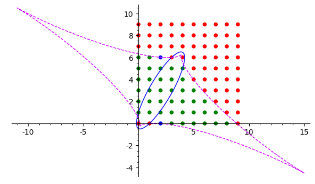
§ and check
with CoCalc Jupyter to help visualize the distribution of locations giving
4 roots (green), 2 roots (red), and 3 roots (the two blue dots, right on the
EVOLUTE).
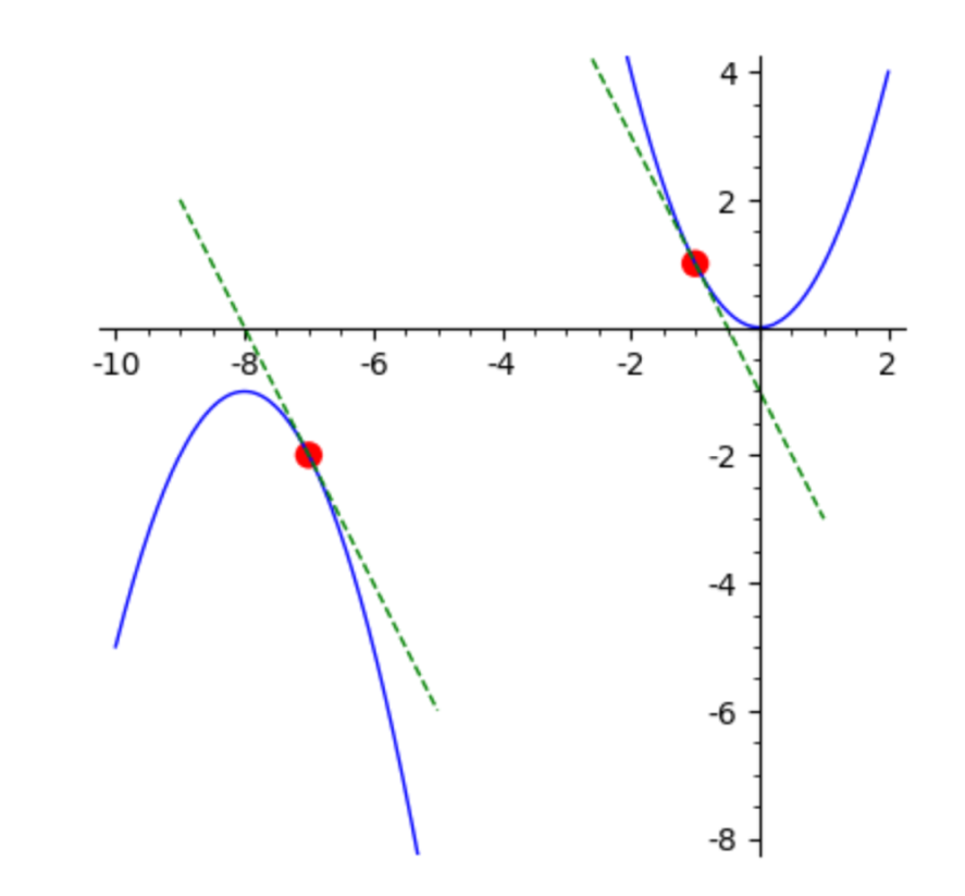
·
Supplementary
Notes on another application of differentiation: To find the closest points
between two parabolas, and
check
with CoCalc Jupyter and its pre-recorded
lecture video.
·
·
Supplementary
Notes to Integration by Parts (pdf file) page 429a-b, with pre-recorded
lecture video.
·
Supplementary
Notes to find area of surface of rotation (pdf file) and check
with CoCalc Jupyter, and its pre-recorded
lecture video.
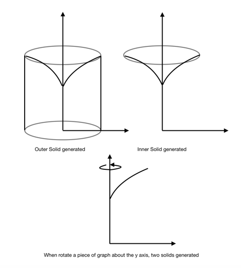
·
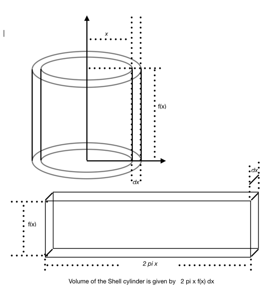
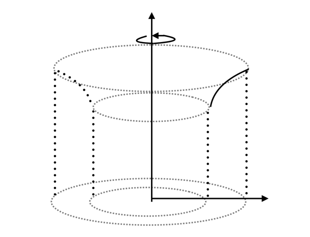
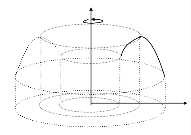
Supplementary
Notes to find volume of “outer solid” of rotation of a graph about y-axis (
Cylindrical Shell Method ) (pdf file) and check
with CoCalc Jupyter, and its pre-recorded
lecture video.
·
Supplementary
Notes on Lines and Planes in 3D and its pre-recorded
lecture video.
·
Supplementary
Notes on another application of linear algebra: To find the 2 by 2 matrix
linear map, and check
with CoCalc Jupyter, and its pre-recorded
lecture video.
·
Supplementary
Notes on another application of linear algebra: To find the closest points
between two lines in 3D, and
check
with CoCalc Jupyter and its pre-recorded
lecture video.
·
Supplementary
Notes on another application of linear algebra: On a simple technique in
cryptography - Hill Cipher, and check
with CoCalc Jupyter, and its pre-recorded
lecture video.
o (you need this for the last question of Assignment 1)
o (you need this for the last question of each of
Assignment 2, 3, 4)
o (you need this if you access CoCalc from a mobile
phone or a tablet computer)
·
Assignments: Students should submit their
solutions of the assignments via Blackboard (under
Content) :
o To do the assignments, first, print out the assignments sheets in hard-copies,
o and write solutions (with formal steps but not rough
work) inside the boxes, and then
o scan solutions into one single clear
and readable PDF file but
o with file size no bigger than 3MB (see
below on usual online technique to reduce pdf file size), and the
o file name must be student’s name
with surname first, and
o the submission must be made by
5:00pm on the due date, with
o a signed covering declaration.
o Solutions must be made within the designated
area (inside the boxes), with detailed workings, presented in a clear, decent,
formal, precise and concise mathematical way, in simple but grammatically
correct English are required. Plan spacing properly, include only steps but not
rough work. Sketch diagrams whenever necessary.
o Please note that only one single submission via
Blackboard will be allowed for each assignment. No other form of submissions
will be accepted (for example, email submissions will not be accepted).
o Only use the app Microsoft Office
Lens to capture images of multiple pages and
make it into one single pdf file (students can also save the file onto PolyU
student OneDrive).
§
App Store for iphone
·
Some popular online web sites for reducing size of pdf
file (file size of each submission should not be exceeding the
file size limit of 3MB)
·
Assignment
1 (a pdf file) Due date 23 Feb 2023 5pm [Thursday week 6].
o
Please
click here
for a suggested solution a few days after the due date.
· Assignment
1a (a pdf file) Due date 2 Mar 2023 5pm [Thursday week 7].
o
Please
click here
for a suggested solution.
·
Assignment
2 (a pdf file) Due date 9 Mar 2023 [Thursday week 8].
o
Please
click here
for a suggested solution a few days after the due date.
·
Assignment
3 (a pdf file) Due date 30 Mar 2023 [Thursday week 11].
o
Please
click here
for a suggested solution a few days after the due date.
·
Assignment
4 (a pdf file) Due date 13 Apr 2023 [Thursday week 13].
o
Please
click here
for a suggested solution a few days after the due date.
·
Three
Practice Questions (no need to submit), and its check
with CoCalc Jupyter.
·
Another
Four Practice Questions (no need to submit), and its check
with CoCalc Jupyter.
·
The Mid-term Test will be scheduled during lecture time in one of the lecture between Week 10 to Week 12. Date and Venue TBA.
o
[and checking Q4a
and Q4b
with CoCalc Jupyter (polynomial long
division, partial fraction)]
o
[and checking the plot of Q7
with CoCalc Jupyter (2D plot)].
o
[and checking Q5c
with CoCalc Jyputer (differentiate symbolically)]
o
[and checking Q2a
with CoCalc Jyputer (implicit differentiation)]
o
[and checking Q4a
with CoCalc Jyputer (curve sketching for rational functions)]
o
[and checking Q6c
with CoCalc Jyputer (integrate symbolically)]
o
[and checking Q2a
with CoCalc Jyputer (integrate symbolically, and binomial coefficients)]
o
[and checking Q3f
with CoCalc Jyputer (integrate and differentiate symbolically, Fundamental
Theorem of Calculus)]
o
[and checking Q1b
with CoCalc Jyputer (area between two curves)]
o
[and checking Q2a
with CoCalc Jyputer (improper integral)]
o
[and checking Q6a
with CoCalc Jyputer (Maclaurin Series, integrate term by term to form another)]
o
[and checking Q2
and Q4 with CoCalc Jyputer (determinant with an unknown, collect polynomial
terms and factorize)]
o
[and checking Q2e
and Q8b with CoCalc Jyputer (eigenvalues, multiplicity, and eigenvectors)]
An open source online software we are using in this subject CoCalc - Collaborative
Calculation and Data Science
·
Demo video on CoCalc part
1
·
Demo video on CoCalc part
2
·
Demo video on CoCalc part
3 and its pdf
print
·
Demo video on CoCalc part
4 and its pdf
print
·
To plot the Batman
Logo a fun way to practice your plotting skills with CoCalc.
The Mathematics
Learning Support Centre
Past Exam Paper
·
2012-2013
Sem 1 Final Exam paper
o
and checking
Q4 with CoCalc Jupyter (implicit plot and plot on the same graph)
·
2012-2013
Sem 2 Final Exam paper
o
and checking
Q12 with CoCalc Jupyter (inverse of a matrix)
·
2013-2014
Sem 1 Final Exam paper
o
Some
Hints and checking
Q5 with CoCalc Jupyter (integration and arc-length)
·
2013-2014
Sem 2 Final Exam paper
o
Some
Hints and checking
Q4 with CoCalc Jupyter (power series)
·
2014-2015
Sem 1 Final Exam paper
o
Suggested
solution to Q1 and checking
with CoCalc Jupyter (derivative)
·
2014-2015
Sem 2 Final Exam paper
o
Suggested
solution to Q1 and checking
with CoCalc Jupyter (arc-length)
·
2015-2016
Sem 1 Final Exam paper
o
and
checking
Q6 with CoCalc Jupyter (step by step row reduction)
·
2015-2016
Sem 2 Final Exam paper
o
and
checking
Q2 with CoCalc Jupyter (power series)
·
2016-2017
Sem 1 Final Exam paper
o
and
checking
Q1 with CoCalc Jupyter (eigenvectors)
·
2016-2017
Sem 2 Final Exam paper
· 2017-2018 Sem 1 Final Exam paper
o
and
checking
Q3 with CoCalc Jupyter (long division of polynomial, partial fraction
expansion, integration)
· 2018-2019 Sem 1 Final Exam paper
o
and
checking
Q2 with CoCalc Jupyter (long division of polynomial, partial fraction
expansion, integration)
· 2018-2019 Sem 2 Final Exam paper Section B
o
and
checking
Q14 with CoCalc Jupyter (integration)
· 2019-2020 Sem 1
Online Final Q1 to Q3 (this file is only showing Q1 to Q3, this was not the
whole assessment item)
· 2019-2020 Sem 1
Online Final Q4 to Q6 (this file is only showing Q4 to Q6, this was not the
whole assessment item)
· 2019-2020 Sem 2
Online Final Exam
o
and
checking
Q7 with CoCalc Jupyter (row reduction)
· 2020-2021 Sem 1
Online Final Exam
·
2020-2021
Sem 2 Online Final Exam
o and checking
Q1 with CoCalc Jupyter (arc-length)
·
2021-2022
Sem 1 Final Exam paper
·
2021-2022
Sem 2 Final Exam paper
·
2022-2023
Sem 1 Final Exam paper
·
Please
note that students may submit their solutions of these past exam papers to
their tutor for markings, and the tutor will then mark and return according to
his/her own schedule.
By: Dr. Heung Wing Joseph
LEE, 李向榮博士
Department of Applied Mathematics, The Hong Kong Polytechnic University.
Email Address: Joseph.Lee@polyu.edu.hk.