MEG experiment on scalar implicature using simple composition paradigm
This is not a real paper; it is an informal writeup of an unpublished experiment. The research was conducted in 2014 at New York University Abu Dhabi, and this report was written in 2015. See My file drawer for an explanation of why I'm recording this. Comments and questions are welcome. —Stephen Politzer-Ahles
1 Introduction
The purpose of this study was to test for neural correlates of scalar inferencing using a paradigm similar to the "simple composition" paradigm of Bemis & Pylkkänen (2011) and many subsequent studies from this group. In the present experiment, participants first saw a target quantifier and then saw two different arrays of dots, and then had to choose the dot array that matched the quantifier they had seen. For instance, in the example below the participant would have to choose the box on the right, in which some of the dots are filled in:
Whereas in the example below, the participant would have to choose the box on the left, in which none of the dots are filled in:
The idea here is that when the participant sees the quantifier, she will need to start thinking about what sort of dot array will satisfy it. The experiment included one block made up of trials like those above—i.e., in that block, a contrast was made between some and none, and thus the participant only needs to access the lower-bounded interpretation of some to complete the task (she does not need to make the some +> not all inference to complete the task). Crucially, this block also included some trials like that shown below, in which the upper-bounded interpretation of some is not relevant (the correct choice is the box on the right, and it is only consistent with the lower-bounded interpretation of some).
This block of trials formed the Lower-bounded quantifier condition, which was expected to minimize scalar inferences on some. Neural responses to the quantifier in this block were compared to those in a separate block, the Upper-bounded quantifier condition, in which the contrast was always between some and all, forcing the participant to realize the upper-bounded interpretation. For example, in that block, the correct answer for the following trial is the middle box:
Whereas the correct answer for the following trial is the rightmost box:
In both of these blocks, the critical time-locking event is the appearance of some in a trial; the appearance of the boxes later is there to give the participants a task, but I didn't look at the MEG data time-locked to that event. The idea is that in the some vs. none block (the lower-bounded quantifier condition), the task should make participants less likely to compute the inference-based, upper-bounded interpretation of some, whereas they should be more likely to do so in the some vs. all (upper-bounded quantifier condition) block. Then it would just be a matter of probing for brain regions that show increased activity in the latter condition.
The reason the some vs. all (upper-bounded quantifier) blocks had three boxes in each trial, rather than two, is because the task becomes very easy otherwise; if these trials only had an all the dots are colored box and a some but not all of the dots are colored box, then ultimately the participant could complete the experiment by not really thinking about quantities at all; in the lower-bounded quantifier blocks she would just need to click whichever side has color on some trials, and in upper-bounded quantifier blocks click whichever side has white on some trials. So the addition of the third box makes it necessary for participants to more carefully evaluate the interpretation of some in this block.
Finally, a pair of control blocks was also used, to isolate effects of inferencing from other sorts of complexity. It is well-known that the upper-bounded interpretation of some is more complex than the lower-bounded interpretation, and in this paradigm the task was also somewhat more difficult in the corresponding block; thus, it was necessary to create a maximally similar pair of blocks that did not rely on a scalar implicature. To try and do this, I made blocks manipulating the color of boxes. In the "Lower-bounded color" condition (scare quotes intentional, since this is not really lower-bounded, but rather is just a counterpart to the lower-bounded quantifier condition), participants had to focus on the contrast between blue and white:
And in the "Upper-bounded color" condition, they had to focus on the contrast between blue and green:
The [sketchy] idea here was that the blue vs. white condition may be easier, if white is considered "no color" and if participants have an easier time distinguishing between color and no color than between one color and another color. It is a weird comparison, but in fact it's not clear what an appropriate non-implicature comparison would be. (Other options that seem like they would easily fit the design, for example top vs. bottom [referring to a box where the top or bottom group of dots is colored in] are problematic because they trigger ad-hoc quantity inferences [i.e., the top dots are colored in +> the top dots and no other dots are colored in].)
Because the task and design are simple, I did the experiment in both English and Arabic. The only difference in the Arabic version is that the critical quantifiers (and other text on the screen, such as messages between blocks and during practice) appeared in Arabic, of course.
2 Methods
2.1 Participants
13 English speakers and 15 Arabic speakers, tested at NYU Abu Dhabi, approved by NYUAD IRB.
2.2 Procedure
Each block had 68 critical trials (some trials) and 68 filler trials (none or all trials, depending on the condition) to establish the relevant contrast. The blocks were presented in a pseudorandom order such that the first two were always the quantifier blocks and the second two were always the color blocks. Each block was preceded by 4 practice trials.
Each trial began with a fixation cross presented for between 250 and 750 ms, then the critical word (the quantifier or the color word) was presented for 800 ms, then another fixation cross was presented for between 400 and 100 ms (the 100 is not a typo, that is what was in the script; I suspect it should have been 1000, but it is not very important because this is just means that the onset of the next picture was 900-1200 ms into the critical epoch, rather than 1200-1800 ms in), and then the boxes with dots were presented until the participant indicated her response (using a button box). There was then a 1000 ms ITI. Each block was divided into 4 sub-blocks, meaning a participant got 3 breaks (of as long as she wanted) during each block).
Before the experimental session began, participants had their head shapes digitized using a handheld FastSCAN laser scanner (Polhemus, VT, USA), and five magnetic coils were attached (three on the forehead, and one each on the LAP and RAP fiducials) for head localization.
2.3 Data analysis
Data were noise-reduced using the time-shifted PCA algorithm in Meg160 (Kanazawa Institute of Technology). Data were subsequently analyzed using mne-python. Bad channels were excluded from further analysis, and then the continuous MEG was subjected to a 40 Hz low-pass filter and then segmented into epochs from -200 to 1200 ms relative to the stimulus onset. Epochs containing artifact were removed from further analysis based on visual inspection, and the first 10 critical "some" trials in any block were also excluded. Noise covariance matrices were computed based on empty room recordings from the same day as the participants' respective recordings. Participants' headshapes and fidicuals were coregistered to the Freesurfer fsaverage brain using the mne.gui.coregistration GUI, and here ico-4 source spaces and BEMs were computed (using the default settings this GUI had in March 2014). The forward solution was created from this in mne-python using mne.make_forward_solution. The data were analyzed in several different ways: based on all trials without artifact vs. based on all trials in which both there were no artifacts and the participant made a correct behavioral response; using loose orientation constraint vs. using a free orientation constraint; and doing separate analyses for the Arabic- and English-speaking groups vs. combining all their data for a single analysis. So, that's already 8 different analyses (2x2x2). Analyses were also conducted on data processed using the lab's BESA pipeline (described in Politzer-Ahles & Gwilliams, 2015, among others). In the results that follow, I will note which results come from which analyses.
Statistical analysis were conducted using the lab's multi-region analysis implementation, which is documented in other papers. In short, for each ROI I do temporal clustering (Maris & Oostenveld, 2007) and identify the largest cluster and its p-value, and then I do FDR correction (Benjamini & Yekutieli, 2001) across the ROIs. I did this two ways. In the factorial analysis, I did a 2x2 ANOVA-like analysis for the spatiotemporal clustering, using a test statistic defined to be largest when there is an interaction such that there is a big effect for the quantifier blocks and a small effect for the color blocks (this test statistic is documented in other papers from this lab, such as Bemis & Pylkkänen, 2011, and Politzer-Ahles & Gwilliams, 2015). In the t-test analysis, for the temporal clustering I just ignored the color blocks and instead directly compared the quantifier conditions using paired t-tests. The rationale for this t-test analysis was that it's unclear (as discussed above) whether the color blocks were really the best non-implicature control comparison, and thus for exploratory purposes I wanted to examine effects of the inference-supporting (upper-bounded) vs. inference-nonsupporting (lower-bounded) quantifier contexts regardless of the control comparison.
3 Results
In the English speaker data and the combined group data, when analyzed through BESA, there was greater activity for the inference-supporting (upper-bounded) quantifier block than the inference-nonsupporting (lower-bounded) quantifier block, and no corresponding difference for the color block, in right BA 42 (transverse temporal, auditory cortex), as evidenced by a significant interaction cluster. This effect, however, did not emerge in the MNE analysis, or in Arabic speakers under any analysis.
In Arabic speakers analyzed through MNE with a loose orientation constraint, there was less activity for the inference-supporting (upper-bounded) quantifier block than the inference-nonsupporting (lower-bounded) quantifier block in left BA 41/42 (transverse temporal, auditory cortex); this effect did not emerge in the other analyses. Also note that this is based on a pairwise t-test; there was not a significant interaction with the quantifier vs. color manipulation for this analysis (although when I divide up the conditions anyway, I get the significant t-test in the quantifier conditions but not in the color control conditions).
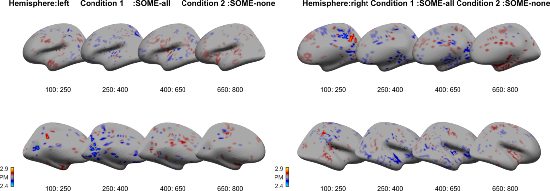
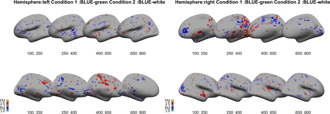
Quantifier data (from the analysis in MNE using a loose orientation constraint and including only trials with correct behavioral responses) for the English speakers are shown below (inference-supporting minus inference-nonsupporting difference, thresholded at p<.01). The top row is the view from the left side (so, the lateral portion of the left hemisphere and the medial portion of the right) and the bottom row is the view from the right side (medial left hemisphere and lateral right hemisphere). Color data are shown below that.


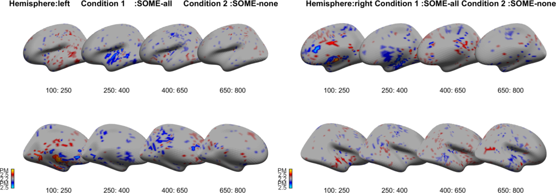
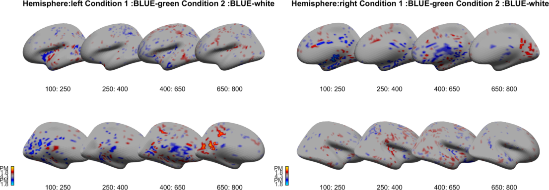
And the corresponding plots for Arabic speakers are shown below.


Finally, sensor-space data showed a numerical trend towards the inference-supporting quantifier context eliciting more negative left-central ERFs around 300-600 ms after quantifier onset than the inference-nonsupporting context did, although this effect did not reach significance.
4 Discussion
As none of the effects observed were very robust across analyses or across language groups, and I did not have a priori expectations for any of the effects to depend on such things, I could not conclude that any of these findings were "real" effects as opposed to spurious patterns. In particular, the strongest effects observed were all near auditory cortex, which was not expected given that the stimuli in the experiment were visual. Note that there is perhaps is reason to believe that superior temporal areas might be involved in scalar inferences, since some theories argue that this "scalar implicature" is actually just a lexical ambiguity (see reviews in, e.g., Sauerland, 2012, and Chemla & Singh, 2014)—but BA 41/42 is probably more posterior than one would expect "lexical" effects to be happening in. (Furthermore, if scalar implicature effects were based on greater lexical ambiguity, or trying to access the less dominant lexical meaning, then one might expect the effects to appear in more frontal areas, as was the case in Shetreet et al., 2013, and Politzer-Ahles & Gwilliams, 2015.) In fact, if previously-reported neurophysiological effects related to scalar implicature are based on resolving ambiguity, then it may not be surprising that no effect emerged in this experiment, since each context strongly biases some towards one reading or the other; on the other hand, if lexical ambiguity is the locus of the effect, then such an effect might only emerge when comparing a strongly biasing context versus a neutral or weakly biasing context, as in Politzer-Ahles & Gwilliams, 2015.
Supporting files
- MEG data: available on request
- Presentation script (.zip file; there are no physical stimuli to provide, because the boxes and dots were procedurally generated, but if you have Presentation this script will work almost straight out of the box, modulo hardware-related changes [setting it up to handle your response devices and output port]; to run it, you just need to enter a subject name which consists of a subject identifier, a list number from 1 to 4, and "english" or "arabic", delimited by underscores, e.g. "subj001_1_english" or "subj007_3_arabic")