The kind of experiment you did at the beginning of the module is called an identification experiment. Another kind of experiment, which is actually much better for revealing how people's minds organize sounds into categories, is a discrimination experiment. Learn how discrimination experiments work by completing the task below; then, in the class discussion section, teach the rest of the class about discrimination (by having them do a discrimination experiment themselves) and have them brainstorm reasons why it is better than identification.
Shortcomings of identification experiments
There are many possible criticisms for the experiment we did before, and the line of reasoning I used.
One major criticism is that in the experiment you did a forced-choice task. In other words, I forced you to choose whether the sound was "pa" or "ba". In the instructions I gave, I did not give you the option of making a response like "this sounded halfway between pa and ba" or "this sounded 80% like a pa, but 20% like a ba". Therefore, maybe it's not surprising that the results looked so categorical; I forced you to have results like that, because I forced you to make an all-or-nothing decision about each sound. Maybe in reality you did notice that sounds with shorter voice onset time sounded less "pa"-like (or they sounded like bad pronunciations of "pa"), but you didn't have the opportunity to indicate that in your answer.
Another problem is mathematical. I suggested before that the results were "categorical" because the line was curved instead of straight. However, it is mathematically guaranteed that this experiment will always create a curved line. Recall the original prediction I made:
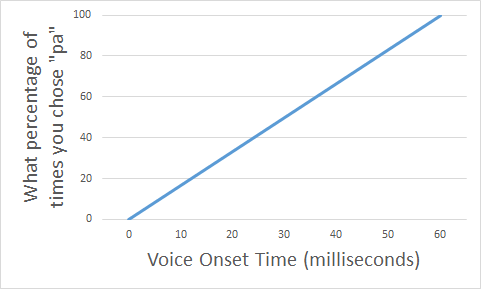
According to this prediction, every time VOT increases by 10 milliseconds, percentage of "pa" response will increase by the same amount. But I arbitrarily chose to test VOTs from 0 to 60. If I wanted, I could have done the experiment with even longer VOTs, and with even shorter VOTs (VOTs below zero milliseconds are possible; those occur in "prevoiced" sounds, where the vocal folds start vibrating even when your mouth is still closed). If I did that, the prediction might look like this:
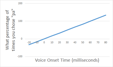
A prediction like this is clearly impossible. This graph is predicting that at long VOTs you will choose "pa" more than 100% of the time (which is not possible; the maximum possible is 100%; it's not possible for you to choose "pa" 5 times if you only hear 4 sounds!) and at short VOTs you will choose "pa" less than 0% of the time (which is, again, not possible).
Because of the nature of the experiment, your results will always be between 0 and 100%. So if we revise the prediction to only have physically possible results, we get something like this:
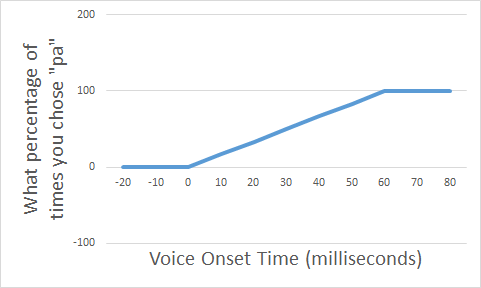
So even now, we have a line that's not straight. Because the line can never go above 100 or below 0, it can never be straight (unless it's straightly horizontal).
In fact, if I stretch the graph a little (not changing the actual data, just changing the shape of the graph I show), it looks pretty similar to the "categorical" results we got:
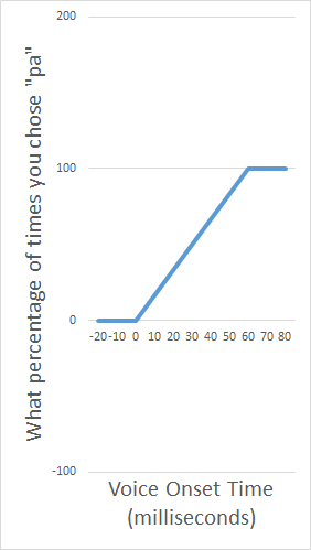
The results might look even more "categorical" if we tested a wider range of VOTs (e.g., down to -100 and up to +200).
So the bottom line is, checking to see whether the line is "straight" is not enough to prove that perception is categorical. In fact the line in our results will never be "straight". And how "curved" the line is depends mainly on how we choose to look at the graph, and how many VOTs we choose to use in our experiment.
So we need another kind of experiment to test categorical perception.
The first experiment you did was called an identificaton experiment, because you had to hear a sound and then identify what sound you think it was. Now we will instead do something called a discrimination experiment, where you have to hear two sounds and try to discriminate (tell the difference) between them.
Here, you are going to do this experiment on yourself, just like you did the other experiment previously.
Make sure you carefully read all the instructions below before you begin.
Categorical discrimination experiment demo
Download experiment files and save them on your computer
- Sound file
- You don't need to download a new Excel file; use the same file you used in the last experiment. It has another tab at the bottom, called "discrimination". Go to that tab.
Understand the experiment procedure
This experiment is almost the same as the previous one, with one difference. In this experiment, instead of hearing single sounds, you will hear pairs of sounds. In the previous experiment you did, you would hear something like "ba...ba....pa....ba...pa...pa...". But in this experiment, you will hear something like "ba ba.........pa ba........ba ba.........ba ba......ba pa......"
Your task is to listen to each pair, and write down whether you think the pair is the exact same sound or different sounds.
(You might hear two sounds that are both "pa" but different recordings of "pa". For example, you might hear a very aspirated/breathy "pa" with a long VOT, paired with a shorter "pa". For those, you should write "different". Only write "same" if you think the two sounds you heard are literally the exact same recording.)
The sound file you downloaded has 55 sound pairs in it. For each pair you hear, write "same" or "different" (or, to save time, you could just write "s" or "d"). You can use the Excel sheet I provided for that (use the tab labelled "Discrimination"); you can record your responses directly on the computer, or you can print out the Excel sheet and write on it, or you can write on any sheet of paper.
The sounds come pretty quickly; there's only a couple seconds of quiet time between each sound. So, once you start playing the file, you should be ready to pay close attention and respond quickly. Make sure there are no distractions around you.
Please do not pause the file, backtrack, re-listen to any sounds, or change any of your answers. Do the whole experiment in one sitting (it will only take a minute).
Do the experiment
Once you've understood the procedure described above, do the experiment. Play the sound file, and write down your answers.
When it is over, you should have 55 responses written down. (If you have more or less, that means you made a mistake. If so, try it again.)
Then you are done with this task. Save your answers, because you will need to analyze them later. But first, let's move on to the next task and learn about some basic concepts that will help you understand the experiment you just did.
Analyze your results
Here we are interested in how often you correctly heard when two sounds are different. In this experiment, 30 pairs really were the same, but 25 pairs were made up of two different sounds. Here are the relevant pairs:
- Pairs with a 0-ms and a 10-ms sound: 12, 21, 36, 37, 47
- Pairs with a 10-ms and a 20-ms sound: 8, 29, 31, 46, 48
- Pairs with a 20-ms and a 30-ms sound: 18, 33, 44, 49, 53
- Pairs with a 30-ms and a 40-ms sound: 27, 34, 41, 43, 54
- Pairs with a 40-ms and a 50-ms sound: 17, 22, 30, 35, 40
For each of these conditions, count how many (out of five possible) pairs you labeled as "different". Convert that number into a percentage (0%, 20%, 40%, 60%, 80%, or 100%). As with the identification experiment, other students' results are compilted in our shared Google spreadsheet, in the "Discrimination experiment" tab.
What do we learn from categorical discrimination?
Remember, all the pairs you counted above were really different; in each of these pairs, you heard two different sounds, with different VOTs. If you are perfect at hearing small differences between sounds, you should have been 100% accurate at saying "Different" for every pair, as shown in the graph below:
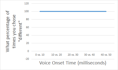
Did your results actually look like that?
If your results look different, what's different about them? Is there anything systematic about your results? Are there certain pairs that you were more accurate with (i.e., more likely to correctly identify as "different) than other pairs?
In reality, people's results often look something like this:
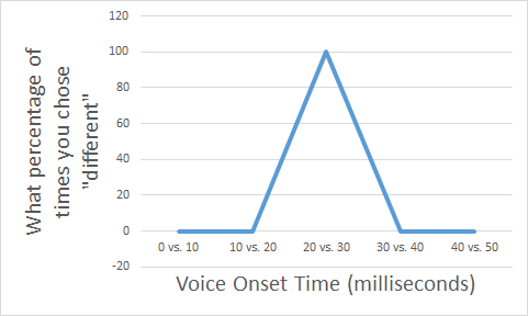
In this graph, the person is perfect at hearing the difference between sounds with 20 ms VOT and 30 ms VOT, but terrible at hearing the difference between any other pairs of sounds.
Were your results like this?
Why might this occur?
Recall that in our discussion of the identification experiment, I suggested that each person might have a categorical boundary. Specifically, I suggested that maybe if my categorical boundary is somewhere between 20 ms and 30 ms, then every sound below that sounds like "ba", and every sound above it sounds like "pa". What consequences will that have when we hear sounds?
Remember that we heard the following kinds of sounds:
- 0 milliseconds of voice onset time;
- 10 milliseconds of voice onset time;
- 20 milliseconds of voice onset time;
- 30 milliseconds of voice onset time;
- 40 milliseconds of voice onset time;
- 50 milliseconds of voice onset time.
Now how might we categorize these when we hear them? If my prediction was right; everything 20 ms or lower will sound like "ba", and everything 30 or higher will sound like "pa":
- 0 milliseconds of voice onset time - sounds like "ba"
- 10 milliseconds of voice onset time - sounds like "ba"
- 20 milliseconds of voice onset time - sounds like "ba"
- 30 milliseconds of voice onset time - sounds like "pa"
- 40 milliseconds of voice onset time - sounds like "pa"
- 50 milliseconds of voice onset time - sounds like "pa"
And when my language system wants to process these sounds, maybe it stops caring about what the exact voice onset time is. Maybe it only cares about the category label: whether this sound was a "ba" or a "pa". After that, this group of sounds might look like this, from the perspective of the language system in my mind:
- "ba"
- "ba"
- "ba"
- "pa"
- "pa"
- "pa"
This would explain the pattern of results. When we hear a 0 ms VOT sound and a 10 ms VOT sound, our mind doesn't really process them as having different VOTs. Instead, it hears the 0 ms sound and thinks, "that's a 'ba'!" Then it hears the 10 ms sound and thinks "that's a 'ba'!" In the end, it doesn't keep track of the exact VOTs anymore, so there's no way to know that the sounds were different. When you are making your same-or-different decision, the only information you have available is: "I heard a 'ba', and then I heard a 'ba'." So you decide that they are the same.
This is the logic of a discrimination experiment. It gives stronger evidence for the presence of categorical perception than the identification experiment can. First of all, it doesn't require you to consciously decide if a sound is 'ba' or 'pa'. Remember that in the identification experiment, I forced you to label every sound as 'ba' or 'pa'; I didn't allow you to write "that was kind of like 'pa' but not a very perfect pronunciation". In this experiment, however, I didn't force you to do that. If you can hear subtle differences between VOTs, it would be possible for you to notice that the 50-ms "pa" and the 40-ms "pa" are slightly different (you might hear that the 50-ms one is "breathier", or sounds more like "pa", than the 40-ms one is) and write down "different" accordingly. But if you write down "same", that gives really strong evidence that you actually didn't notice the difference between different VOTs, even when you had the chance to.
The discrimination experiment also gives us an easy way to identify the categorical boundary: the place where there's a "peak" in the graph. For example, in the example above, the "peak" was at the 20-vs-30 comparison. That means that people in that example are best at hearing the difference between 20 and 30 milliseconds of VOT; that suggests that the boundary between "ba" and "pa" must be between 20 and 30 ms for those people.