Analyze your data (1 hour)

↵ Back to module homepage

If you record yourself saying "pa" and "ba" many times, and measure the voice onset time every time, you will probably notice that it varies a lot. Your "pa" won't have the same voice onset time every time you say it. Maybe sometimes it's 85 milliseconds, sometimes 78 milliseconds, sometimes 92.3 milliseconds, etc.

In fact, voice onset time has a wide range. When it's really short (like 1 or 2 milliseconds), that might obviously sound like "ba". When it's really long (like 150 milliseconds), that might obviously sound like "pa". But what will your mind do when it hears voice onset times that are somewhere else in this range? What will a voice onset time of 25 milliseconds sound like? What about a voice onset time of 43 milliseconds? What about 57 milliseconds?

That's what this experiment was about. I used Praat to modify the "pa" that I recorded. While "pa" naturally has a pretty long voice onset time, I can cut parts of it out to make it shorter and shorter. So I artificially created sounds with various voice onset times: 0 milliseconds, 10 milliseconds, 20 milliseconds, etc. I had you listen to those sounds and decide whether they are "ba" or "pa". In this way, we can examine how you understand sounds differently depending on their voice onset time. We might be able to find out how much voice onset time a sound needs for you to think it sounds like "pa".

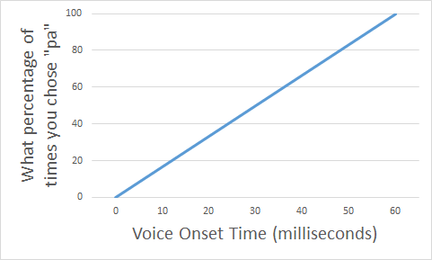
As we discussed before, sounds with short voice onset time sound like "ba", and sounds like long voice onset time sound like "pa". So we might predict that, the longer the voice onset time is, the more it sounds like "pa". If I graph how often you chose "pa" for each voice onset time, I might expect that for sounds with longer voice onset time you chose "pa" more often, as shown in the graph below:

Graph showing how often you choose "pa", as a function of the VOT of the sound you heard. When VOT is low, the percentage of times you choose "pa" is low. As VOT increases, percentage of time you chose "pa" steadily increases, making a straight, upward-sloping line.

Your job now is to analyze your data to see if this prediction was correct. For each Voice Onset Time you heard, you will count up how many times you chose "pa", and make a graph like this. When you are ready, do the task below.

Go back to the results you recorded when you did the experiment. You should have 28 responses (all either "ba" or "pa".

For each VOT, count how many times you wrote "pa". For example, for 30 ms, check #1, #7, #10, and #15. If you wrote "pa" for #7 and "ba" for the other three, then your answer is "1" (you wrote "pa" one time for the 30-ms tokens.

Then, convert these responses into percentage (out of 4). 0 out of 4 is 0%; 1 out of 4 is 25%; 2 out of 4 is 50%; 3 out of 4 is 75%; and 4 out of 4 is 100%.

When I teach this class with a group of students, I like to create a shared Google spreadsheet and have all students input their results into it so they can compare what they found. This is also a useful way to see the general trend across multiple people (for example, if 90% of students were faster for 'related' than for 'unrelated' and 10% of students were faster for 'unrelated' than 'related'), which is important in any empirical research. If you are teaching this class, you can make your own spreadsheet for your students. On the other hand, if you are using this webpage to learn independently, you can visit my class's spreadsheet above to see what some other students found.

Finally, answer the question: Did your results match the prediction I described before? If your results were different than the prediction, describe how they are different.
When you have finished these activities, continue to the next section of the module: "The concept of categorical perception".


by Stephen Politzer-Ahles. Last modified on 2021-07-13. CC-BY-4.0.